+ Reply to Thread
Results 1 to 5 of 5

Dynamic Cascading Drop-Downs Using INDEX & MATCH

  1. #1
    Forum Expert GeneralDisarray's Avatar
    Join Date
    09-15-2011
    Location
    Pittsburgh, PA, USA
    MS-Off Ver
    Windows Excel 2016
    Posts
    1,416

    Dynamic Cascading Drop-Downs Using INDEX & MATCH

    I dug this up after reading Jbeaucaire's thread (link here). This is just another way to solve that problem using Index and Match. I like learning numerous ways to do things like this, if you do too, then please read on.

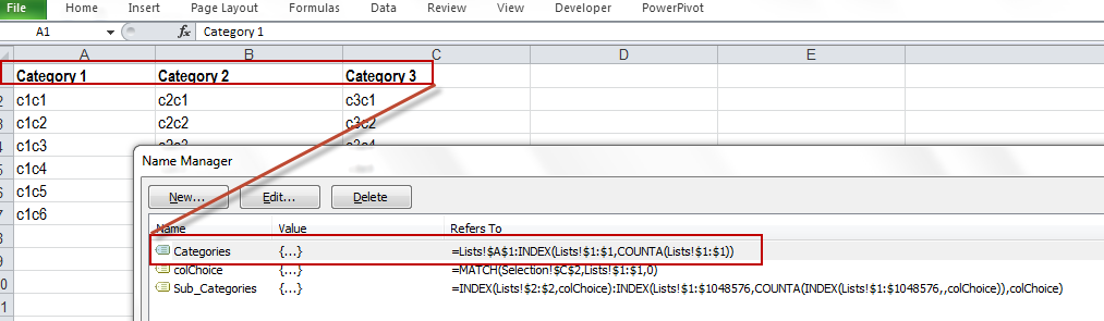
    Create the top Categories as a header row above the associated subcategories (fig1).
    Name:  fig1.png
Views: 9625
Size:  9.8 KB

    TOP CATEGORY (FIRST-DROP-DOWN)
    Create a named range for the top Categories (header row). Using Index, we can create a dynamic range (expands / contracts when you add / remove columns). The Refers-To box for Categories reads
    =Lists!$A$1:INDEX(Lists!$1:$1,COUNTA(Lists!$1:$1))
    Name:  fig2.png
Views: 9729
Size:  42.8 KB

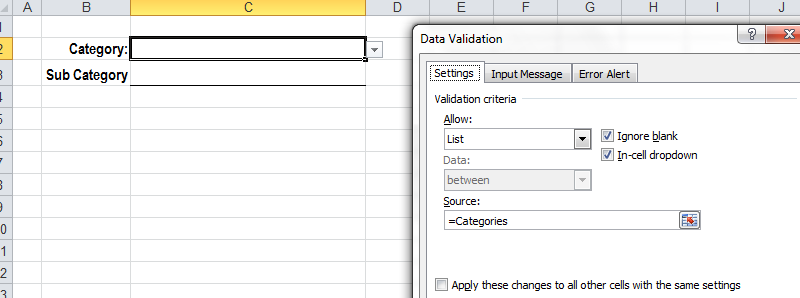
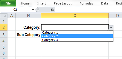
    "Categories" is used in the data validation list source, for the first drop down (fig3 & 4).
    Name:  fig3.png
Views: 9572
Size:  25.9 KB

    Name:  fig4.png
Views: 9685
Size:  15.2 KB


    SUB-CATEGORIES (DEPENDENT-DROP-DOWN)
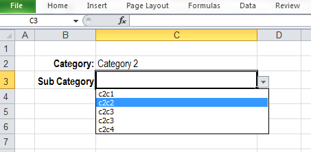
    The second drop down menu, is defined by the users choice in the top category. A second named range, Sub_Categories provides the dynamic range needed for that data validation list (fig5)
    Name:  fig5.png
Views: 9818
Size:  15.1 KB

    The data validation for this cell is similar to the top category drop down, it is simply the name "sub_categories" (sorry, only 5 figures per posting).

    In this version of the solution, the named formulas do the work. As shown in fig2, Sub_Categories makes use of the index function to define a subset of a column. The Refers To field for Sub_Categories reads:

    =INDEX(Lists!$2:$2,colChoice):INDEX(Lists!$1:$1048576,COUNTA(INDEX(Lists!$1:$1048576,,colChoice)),colChoice)

    colChoice is a third named formula, added just to make sub_categories more readable. colChoice is a standard use of the Match function used to "match" the users top category selection with the corresponding column on the "Lists" worksheet (also shown in fig2).
    colChoice = Match(Selection!$C$2,Lists!$1:$1,0)


    If you are unfamiliar with the INDEX function, this may look a little confusing. The main idea is, the first instance of the Index function (to the left of the Colon operator), defines a single cell reference corresponding to the top of the selected choices (note, this the choices start in row 2). In this example, it will place return A2, B2, or C2.

    The second and third instances are a bit trickier, but they function to return a reference to the bottom cell (last) of the appropriate column. They will evaluate to either A7, B6, or C10 in this example. The entire formula will return one of the following (again, in this example) A2:A7, B2:B6, or C2:C10. Note, if you add or remove choices from any of the list, this function will expand/contract to reflect the change!

    For a very good explanation of INDEX used to create named formulas, read up here.

    My example is attached to the next post
    Last edited by GeneralDisarray; 07-07-2012 at 07:47 AM. Reason: typo fix
    Remember, saying thanks only takes a second or two. Click the star icon(*) below the post you liked, to give some Rep if you think an answer deserves it.

    Please,mark your thread [SOLVED] if you received your answer.

  2. #2
    Forum Expert GeneralDisarray's Avatar
    Join Date
    09-15-2011
    Location
    Pittsburgh, PA, USA
    MS-Off Ver
    Windows Excel 2016
    Posts
    1,416

    Re: Dynamic Cascading Drop-Downs Using INDEX & MATCH

    attachment for described solution.
    Attached Files Attached Files

  3. #3
    Forum Guru TMS's Avatar
    Join Date
    07-15-2010
    Location
    The Great City of Manchester, NW England ;-)
    MS-Off Ver
    MSO 2007,2010,365
    Posts
    44,336

    Re: Dynamic Cascading Drop-Downs Using INDEX & MATCH

    Instead of:

    Lists!$1:$1048576

    why not:

    Lists!$A:$A


    Regards, TMS
    Trevor Shuttleworth - Retired Excel/VBA Consultant

    I dream of a better world where chickens can cross the road without having their motives questioned

    'Being unapologetic means never having to say you're sorry' John Cooper Clarke


  4. #4
    Forum Expert GeneralDisarray's Avatar
    Join Date
    09-15-2011
    Location
    Pittsburgh, PA, USA
    MS-Off Ver
    Windows Excel 2016
    Posts
    1,416

    Re: Dynamic Cascading Drop-Downs Using INDEX & MATCH

    Well, let me break this down the second index third INDEX function:

    First off, I'm using index with three arguments (Table, Row, Column) to return a reference to a cell. The reference will bottom-out my second drop down menu. The overall goal is to return a reference to the bottom-most cell of the column matching the user's choice (from the first drop down).

    =INDEX(Lists!$2:$2,colChoice):INDEX(Lists!$1:$1048576,COUNTA(INDEX(Lists!$1:$1048576,,colChoice)),colChoice)


    Table argument(Lists!$1:$1048576)
    The table I'm interested in sits in the Lists worksheet, and I don't know how many rows and columns will be used. To allow for and unknown number of columns, I'll just assume the table starts in the upper left cell and pass in the entire sheet. That's what the Lists!$1:$1048576 does for us, it passes in all rows (entire-rows).

    The second use of the index function highlighted in blue, returns an entire column (the one matching the users selection "colChoice"). By leaving the row argument blank (INDEX(Lists!$1:$1048576,,colChoice)) - we tell index to return the entire column.

    In words: INDEX(Lists!$1:$1048576,,colChoice) means "return to me the entire column from the worksheet named list, whose column number is colChoice". By including that entire column in the COUNTA() function, we return the count of non-blank cells in the colChoice column (Since the column starts in the first row, this count is the row number of the bottom-most cells we are looking for -- assuming we have no blanks in the drop-down menu. A safe assumption if we build the list in the first place with that in mind).

    SO, this blue highlighted section returns the row number we need.

    Putting this together, we have:

    =INDEX(Lists!$2:$2,colChoice):INDEX(from-entire-Lists-worksheet, Bottom-most-row#-with-text-in-colChoice-column, colChoice-column#)

    And since we have indexed the entire sheet, we will get a reference like cells(bottom-row,choosen-column).address on the right side of the colon operator to complete our drop-down list
    Last edited by GeneralDisarray; 07-16-2012 at 11:51 AM.

  5. #5
    Registered User
    Join Date
    11-07-2013
    Location
    Derbyshire, England
    MS-Off Ver
    Excel 2016
    Posts
    52

    Re: Dynamic Cascading Drop-Downs Using INDEX & MATCH

    This is great and I want to be able to use this system.

    But!

    How do I expand it so as when I am on the next line down I can make an independent selection.
    In the part "colChoice = Match(Selection!$C$2,Lists!$1:$1,0)" I need this to work in the next row down 5000 rows
    e.g.
    colChoice = Match(Selection!$C$3,Lists!$1:$1,0)
    colChoice = Match(Selection!$C$4,Lists!$1:$1,0)
    colChoice = Match(Selection!$C$5,Lists!$1:$1,0)

    How can I edit this without having an independent colChoice in name manager for each row?
    Attached Files Attached Files

+ Reply to Thread

Thread Information

Users Browsing this Thread

There are currently 1 users browsing this thread. (0 members and 1 guests)

Bookmarks

Posting Permissions

  • You may not post new threads
  • You may not post replies
  • You may not post attachments
  • You may not edit your posts

Search Engine Friendly URLs by vBSEO 3.6.0 RC 1